Alle links
Gymnasie links
Andre links
Regler
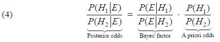
Faglig forening
Turing's attack on the Vigenère CipherOn my Enigma-page it was mentioned how statistical methods were used during World War 2 in order to break the Naval Enigma M3. The process was named Banburismus. Because of the complex theory behind the statistics used in Banburismus, I have decided to describe another of Alan Turing's methods, namely his attack on the Vigenère cipher. This will allow us to look more closely at the mathematics involved. The method is described in his theoretical article The Application of Probability to Cryptography (se [1]) written during WW2, but first released for the public in 2012. The article contains four situations in which Bayes' formula can be used to reveal strong information from the encrypted text. Those four topics are: The Vigenère Cipher, A letter subtractor problem, Theory of repeats and finally Transposition ciphers.
1. Use of statistics in cryptography historicallyIt is well-known that the early monoalphabetic substition ciphers, where each letter is encrypted to another unique letter, could easily be broken by using statistics. If the encrypted text is sufficiently long, one can be (almost) sure that the letter appearing the most often, will be the encryption of an E in clear text. When the Vigenère Cipher was invented, it became harder, because the letter frequencies were "smoothened out" so to say. But also here the cryptographers came up with a solution. The Mayor Friedrich Kasiski (1805-1881) contributed, but especially William F. Friedman (1891-1969) invented a usefull tool in the work of breaking the Vigenère Cipher: Index of Coincidence. The reader is encouraged to find more about this elsewhere. These methods all rely on the fact that the frequencies of letters occuring in a normal text are different. If the frequencies were all equal, those methods would not work! The same is the case for Alan Turing's methods. The difference is however that Alan Turing is extracting more information from the evidence (the encrypted text). This makes his method the strongest.
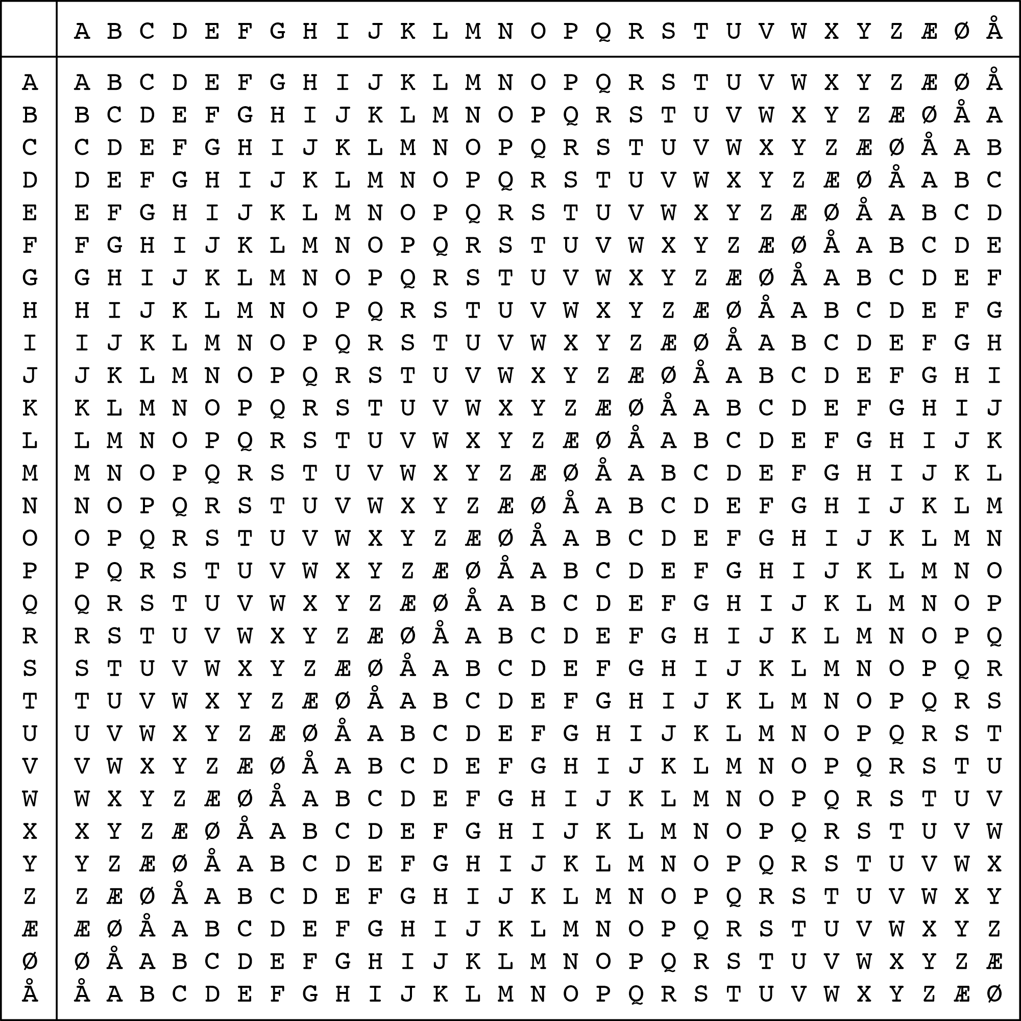
2. The Vigenère Cipher explained brieflyLet's look at the properties of the Vigenère Cipher. Firstly it is a polyalphabetic system, meaning that it is using several substitution alphabets. For the Vigenère Cipher a secret Key (or Key-word) is telling what alphabets are being used and when. Let's look at an example. The starting point is the table below (Click for a bigger table):
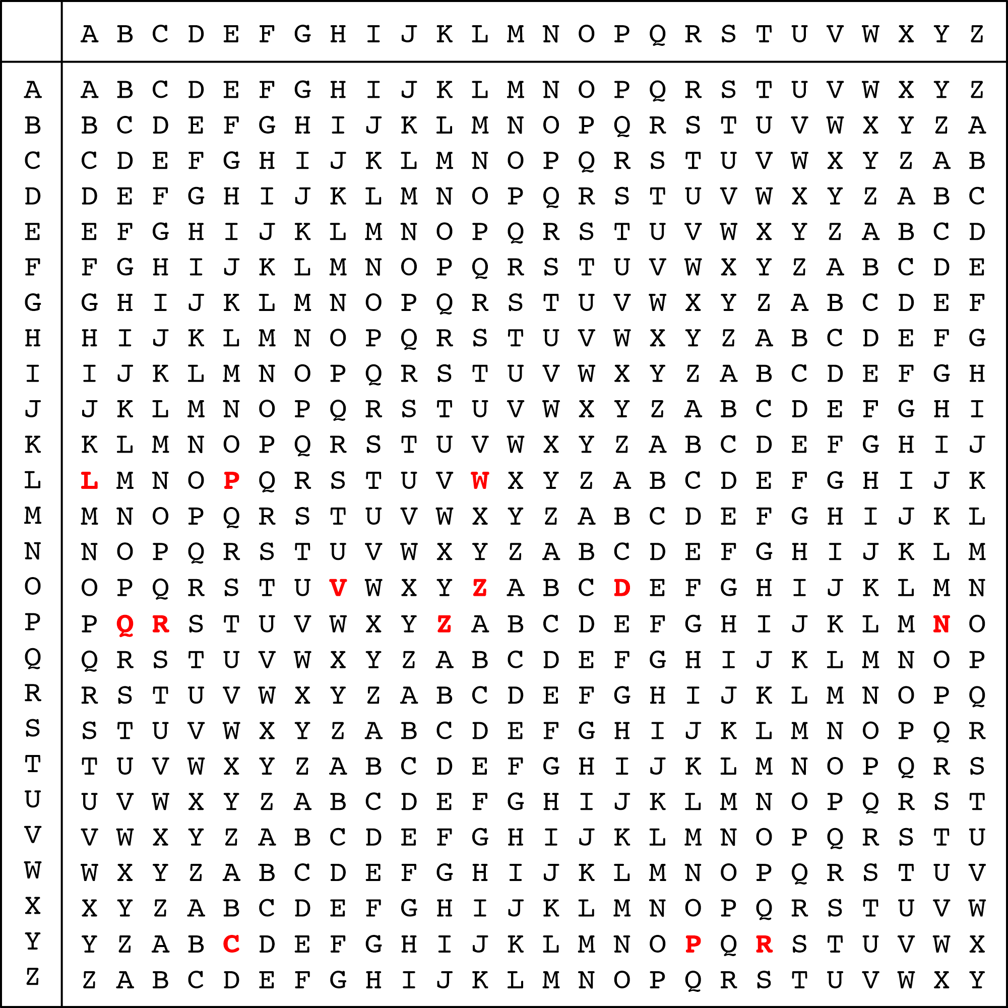
Let's say that the secret key-word is POLY and that we want to encrypt the cleartext BLETCHLEYPARK. We take the first letter in the cleartext which is a B and the first letter in the key, which is a P. By looking up B in the upper row and P in the left column of the table, we find that B is encrypted as Q. Next letter in the cleartext is L and the next letter in the key is an O. Again we find L in the upper row and O in the left column to find that L encrypts to Z. We continue this way: E encypts
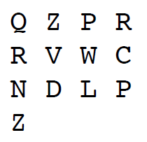
to P an T encrypts to R. Now we have come to the end of the key-word and begin over again: Finding C in the upper row and P in the left column tells us that C encrypts to R. Continuing this way we end up with the cleartext BLETCHLEYPARK being encrypted into QZPRRVWCNDLPZ. In the table below the actual letters from the encrypted text is shown in bold red.
We can arrange the encrypted text i rows of 4 letters, corresponding to the fact that the length of the key-word is 4. We realize the advantage by this representation: Each column have been encrypted using the same alphabet! So the same letter in the key-word has been used.
This means that we are back in the situation with a simple monoalfabetic system, which can easily be broken - if each column is suffciently long. This obviously is not the case here. We have a maximum of four letters to produce statistics on! Another problem is to determine the length of the key-word. The key-word is normally unknown! Without it we would be unable to make the arrangement above. It is however here that Friedman come to our rescue. With his Index of Coincidence we would be able to receive a good bid on the length of the key-word.
3. Alan Turing's exampleIn his article The Application of Probability to Cryptography (see [1]) You might even want to watch [3], including comments by Sandy Zabell. Alan Turing is looking at the following encrypted text: DKQHSHZMNPRCVXUHTEAQXHPUEPPSBKTWUJAGDYOJTHWCY-DZHGAPZKOXOEYAEBOKBUBPIKRWWACEJPHLPTUZYFHLRYC Here - means continuation on next line. We know that the Vigenère Cipher has been used for encryption. In the following sections we will look at how the Friedman Test along with the application of simple statistics will do in the decryption process compared to how Alan Turings method involving Bayes' Formula will do the job. To keep the record, we will at this place deliver the cleartext along with the secret key-word. In the following sections this knowledge should however be considered unknown. Secret key: POIUMOLQNY Cleartext: OWINGTOWARCONDITIONSITHASBECOMEIMPOSSIBLETOIMPORT-CALCULATINGMACHINESXTHISISVERYREGRETTABLE
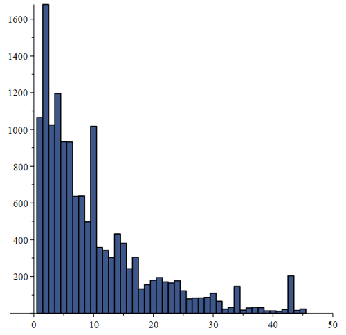
4. Application of the Friedman Test and simple statisticsBelow we are delivering the result of applying the Friedman Test to Alan Turing's example from section 3, without any details. The appropriate tool is the Index of Coincidence. The interested reader, who would like to know more about this test, is encouraged to consult Wikipedia.
The column over 10 on the 1. axis is especially high, which indicates that 10 could be a good bid for the length of the key-word. We will go with that value in the following. As indicated in section 2 it is useful to organize the encrypted text i rows of 10 letters, corresponding to the length od the key-word. .
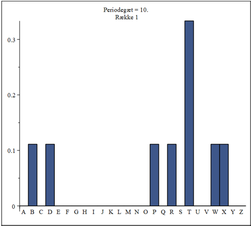
In this "red matrix" we now know that letters in the same column are encrypted using the same alphabet (substitution). The key-word is still unknown, only it's length is known. Our job will be to determine the key-letter in each column. When that is done, one can easily complete the decryption. In the following we will be using statistics on each column. Let's look at the first column. Without details we receive the following histogram for the letter frequencies in the first column:
The statistics is obviously bad - too few letters in each column to give anything significant! The histogram suggest the letter T to be the encryption of the letter E, because this column is the highest. Looking in the Vigenère table, we see, that IF the key-letter is P, T will endeed be the encryption of E. From our knowledge from section 3, we know that P is indeed the correct key-letter, so here this simple statistics got it right. Now, let's look at column 2:
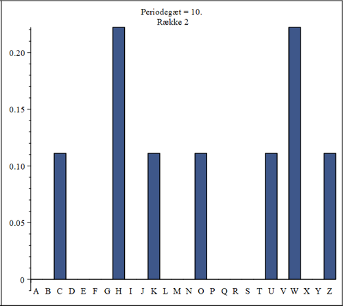
The highest columns in this histogram is H and W. If one of those letters should be the encryption of E, then the second letter in the key-word need to be either D or S, which is not the case. The column over S should have been the highest, but it is empty. We conclude that the simple statistics doesn't work in this case. Continuing in that way, we realize that the simple statistics only hit the correct letter (for the encryption of E) in two columns out of 10. We conlude that this simple statistical approach isn't good, when the encrypted text is too short (especielly the length of the columns). At least it would require a lot of guess-work and testing to continue along that road.
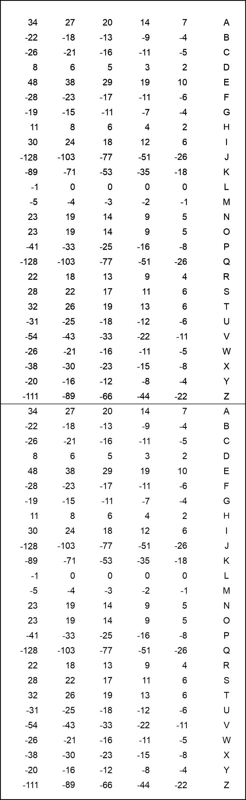
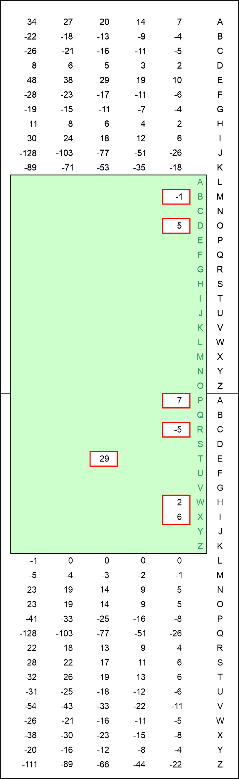
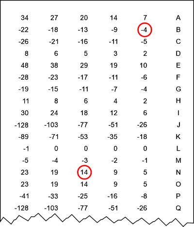
5. Alan Turing's method in useIn this section we will investigate how well Alan Turing's method does the job. We will however assume, that we beforehand have been using the Friedman Test in order to give us the length of the key-word, which is 10. Below I will explain the method without initial details. The theoretical explanations will be postponed to later sections. We will need a "score-table" (click on the image for a bigger version):
The explanation how the values in this score-table has been calculated will be postponed to later sections. The unit for the scoring values in the table is half decibans, which will be defined in section 8. We don't need it at this moment. Let's look at the letters in the first row of the "red matrix" in the previous section: DRXTTPBWT. The letters D, R, X, P, B, W all occur one time, whereas the letter T is occuring three times. We now create a "slider", which could be a piece of paper with holes. We cut holes in the slider beside the letters mentioned above, in the following way: If a letter is occuring only one time, the hole should be right over the number-column to the far right. If a letter is occuring two times, the hole is supposed to be cut over the second number column, counted from right towards left. Is a letter occuring three times, the hole should be cut above the third number-column, again counted from right towards left, etc. In the actual situation the green slider is displayed on the figure below (click for a bigger version):
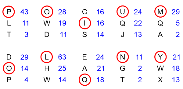
The idea is now to slide the green slider up and down until the sum of the scoring values, which can be seen through the holes, reaches a maximum. The above figure show the slider in the position with the biggest sum: 43 half decibans. The letter beside A in the letter-column to the far right then is a good bid for the key-letter corresponding to the first column. It is a P here. From our knowledge from section 2, we know this to be correct! The same procedure is executed for every column in the "red matrix". The result is shown on the figure below. For every column we have written the three letters with the highest scores (in half decibans).
We notice that in 7 out of the 10 columns the correct key-letter will be the letter with the highest score. In two cases it is the letter with the second highest score, and in one case the correct key-letter is the letter with the third highest score. The different scoring values are placed in blue to the right of the individual letters. The values for the three letters with the highest scores are not that different here. Had the text just been a little longer one would often see the highest score being significantly higher than the second highest score. Often negative values will appear already for the letter with the second highest score. Anyway we conclude that Turing's procedure is significantly better that using simple statistics. The reason is the fact that Alan Turing's method is extracting much more information from the data or evidence at hand (the encrypted text). It will however still be necessary to make a few trial and errors, to receive the correct key-word. When this word is found, the cleartext can easily be determined. In the following sections we will be looking at the theory behind the method devised by Alan Turing. The attentive reader may wonder why the scoring values from A to Z has been "doubled" vertically. This is of practical reasons: when using the slider this means we can easily "go around the clock" instead of starting all over again from the beginning of the alphabet from A to Z ... P.S.! It should be mentioned that some of the values in the scoring table, which I have shown above, are slightly different from the table, which Alan Turing is using on figure 3 on page 7 in his article [1]. Maybe Alan Turing did some rounding-off in his manual calculations? Anyway the small differences really doesn't matter.
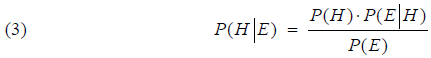
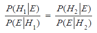
6. Bayes' Formula on relative odds formAs mentioned earlier the statistical method developed by Alan Turing is building on Bayes' formula from Probability Theory. In the following we will se how Bayes' formula come into play. I will be a bit brief on the first part dealing with well-known relations. Let H and E be two events in a finite Probability Space. Assuming P(E) is different from 0, the conditional probability for H given E is defined as follows:
Due to symmetry we have:
from which we get the simple version of Bayes' formula :
The deeper meaning of Bayes' formula is the fact that it relates a conditional probability to the same conditional probability, just with the events swapped. Given two events (hypotheses) H1 og H2, we can use Bayes' formula (3) on each of them, given the same evidence E, thereby creating a new formula named Bayes' formula on relative odds form.
The so-called Bayes factor is the proportion between the probabilities for seeing the evidence E given the hypotheses H1 and H2 respectively. What we are doing is comparing two hypoteses H1 and H2, starting out with a priori odds for the hypothesis H1 against the hypothesis H2. The content of (4) can then be interpreted in the way that we get the "updated" or posterior odds (after taking into account the evidence E) for the hypotheses by multiplying the a priori odds by the Bayes' factor.
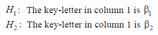
7. Bayes' Formula used on the actual problemWe are going to apply Bayes' Theory on the example in which the evidence E is the encrypted letters in the first column in the "red matrix" in section 4. Our two hypotheses are:
where β1 and β2 are two given letters. Formula (4) above now becomes:
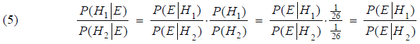
We have here used that all key-letters in the first column are equal likely, hence the a priori odds are (1/26)/(1/26) = 1. The reason is the fact that key-letters can be chosen freely. The key-word doesn't need to mean anything within the Enlish language. The content of (5) now reads: The posteriori odds - after taking the evidence into account (data in the 1. column) - is equal to the Bayes' factor to the far right in (5). The numerator in the Bayes' factor kan be interpreted as the probability of seeing column 1 given that the key-letter is β1. Something similar can be said about the denominator. In the following we want to calculate a matematical expression for the conditional probability in the numerator. Firstly let's denote the encrypted letters in column 1: α1, α2, ... , αi, ... In the actual situation they are equal to D, R, X, T, T, P, B, W, T. Let's for a moment assume, that the key-letter in the 1. column in the "red matrix" in section 4 is a C. If so we get the cleartext by shifting backwards with 2: D is the encryption of B, R is the encryption of P, etc. The (assumed) cleartext corresponding to the 1. column is shown in blue below:
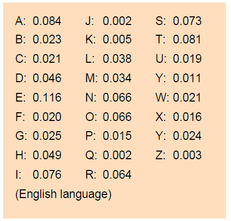
Now what is the probability of seeing column 1 if the key-letter is a C? Well, here we are back in cleartext and can consequently apply the letter-frequencies. Alan Turing used the following values for the letter frequencies for the English language:
It must be considered a very good approximation assuming that the events of getting each of the nine letters in the 1. column are independent events, since there are 10 steps between them in the actual cleartext! This means that the total probability of seeing the 1. column will be the product of the frequency of each letter. We will let Pk denote the frequency of the k'th letter. Hence we get the following expression for the probability of seeing the 1. cloumn when the key-letter is a C:
where we are making the following identifications: A is 1, B is 2, ... , Z is 26. As an example α1 is here equal to D, which we will identify with 4. Subtracting 2 yields 2, which means a B in cleartext. The first factor in the product consequently is the frequency of B in cleartext, which according to Alan Turings frequency table is equal to 0.0023. Similar with the other factors in the product. BUT, the key-letter in column 1 doesn't need to be a C: Actually it is this letter we are searhing for. If it is a general letter β, then the following product will be the probability of seeing column 1 when the key-letter is β (consider this statement!):
implied that E is the evidence (encrypted text in the first column) and H is the hypothesis that the key-letter for the column is β. It would seem an obvious choice to look at the probability P(H|E) in our work on creating the score-table mentioned in section 5. The bigger this conditional probability, the more likely it is, that the key-letter β has been used. The identity (5) shows however, that we can as well swap those two events: The probabilities P(E|Hi) are namely proportional to the probabilities P(Hi|E), as we realize by rewriting (5):
This means that we can as well use the right side of (6) - or something which is proportional to it - in our work on defining a score-table. Alan Turing did choose to multiply with 26 for practical reasons, i. e. he used the following expression as an initial step in his calculations:
CommentsIn his article [1] Alan Turing deliver an expression for the probability β being the correct key-letter given the evidence from column 1:
The probability on the righthand side of (6) has been divided by the sum of probabilities for seeing the column given each of the possible key-letters from A to Z. This formula has its origin in Bayes' formula and the fact that the a priori probabilities are all equal to 1/26. This formula is however not necessary and could confuse our arguments above. Therefore it is only placed here for the matter of completeness.
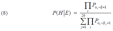
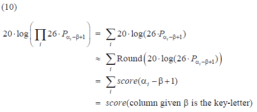
8. Deciban and score-tableAlan Turing realized that it would require a lot of heavy manual work calculating the multiplications in the expression (7). Inspired by the way sound pressure is being defined in Physics using a logarithm, he decided that the score for a letter in the alphabet should be a logarithm of 26 times the letter-frequency in the english language. He used the logarithm with base a = 101/10. The obvious advantage of using a logarithm is the property that it turns multiplication into addition. This would save a lot of time in the manual work. Since all logarithms are proportional we can translate his logarithm with base a = 101/10 to the ordinary logarithm with base 10, log(x):
The unit was named deciban (like decibel). Here ban was inspired by the name of the town Banbury, as mentioned earlier. Later a colleague of Alan Turing, I. J. Good, proposed delivering the scores in half decibans, because it would reduce the time required for practical calculations. The score in half decibans for the k'th letter Pk then was defined as::
Let's look at an example. The score for the 2. letter in the alphabet, B is:
where 0.023 is the frequency of the letter B found in the frequency table above. Notice that the reult was rounded off to the nearest integer. This approximation was sufficiently accurate by any means. If a letter appeared more than one time in the column, one could of course multiply the score for the letter with the number of times it occured, but it was more convenient calculationg the score for all occurences in one go. In addition it would be a bit more accurate, because of the rounding off process. Let's say as an example that the 14. letter in the alphabet, N, is occuring 3 times in a column. This would give the following score:
We just multiply by 3 and round off. A total score of 14 for the three N's. This score was placed in the 3rd number column, counted from right towards left in the score table (see section 5).
By using (7) we are able to calculate the total score (up to rounding) for the entire column, given β is the key-letter:
where again a letter is being identified with it's number in the alphabet. It is left to the reader to convince him/her-self that the technique described in section 5 (using the slider in the score-table) is exactly the same as using the above formula (10) - with the understanding that if a letter occur multiple times, it's total score should be calculated in the way N was treated above.
9. Theory of RepeatsAlan Turing's third example of using his stastistical methods in article [19] is described in his section Theory of repeats. It is probably this section which comes closest to the theory behind the process of Banburismus which took place at Bletchley Park during WW2. This section is dealing with repeats, bigrams, trigrams, etc. It is pretty complicated and scoring tables are missing. Not more about this here.
10. Alan Turing's philosophyAt Bletchley Park Alan Turing was interested in producing decryption methods which worked, not just producing useless theory. Beside being a theorist he was certainly also spokesman for applied math. In his work with Banburismus at Bletchlet Park he wrote: When the whole evidence about some event is taken into account it may be extremely difficult to estimate the probability of the event, even very approximately, and it may be better to form an estimate based on a part of the evidence, so that the probability may be more easily calculated.
11. Literature/links
This page was written July 2023. |
|
|